Introduction

Survival plot is usually a short note. It was asked in December 2019 DNB final theory examination. Let us look at this to understand survival plots which is one of the most common plots we see in oncology trials, and most drug approvals, are based on improvement in various survival times. There are various terms associated with survival analysis.

• Survival analysis: it is a different branch of statistics, that mainly deals with analyzing the outcome of patients till some event of interest occurs, or simply an analysis to estimate the survival of patients in a given set of data

• Survival time is the “statistics that measures time of follow-up from a predefined point of start (i.e., from the time of randomization or diagnosis) to the occurrence of a given event (relapse, progression, or death),”

• Survival plot/survival curve is a term that is “used to represent a group of plots that are constructed based on the time to event data.” It measures the fractions or percentage of patients living for a particular or specific amount of time after randomization, intervention, or treatment.

Q1: How and Why Is Survival Analysis Different from Usual Statistics?

Survival analysis was initially used in trials, where the event was “Death,” however, over time this survival analysis is being used for various indications inclusion, time to onset of disease, time to progression, time to discharge, etc.,

1. The distribution of patients population is very rarely normal

2. All members do not enter the study at the same time, and hence, usually have a different follow up time

3. This dataset usually has censoring (in a few patients, the predefined event of interest may not have occurred till the end of the study) which is usually not the case with usual statistics. Hence, the usual statistical techniques cannot be applied here.

Q2. What Are the Different Types of Survival Analysis and Plots? Advantage and Disadvantages of Various Types?

Different types of survival curves

1. Life table analysis

2. Kaplan–Meier (K-M) survival curve.

Life table analysis

In this method, the total duration of follow-up is divided into intervals of fixed duration. For each of these intervals, calculations are made for those patients who reached the end point (or event). Thus, a proportion is calculated of the patients who had an event to those who were at risk at the beginning of the interval. For each succeeding interval, the same proportions are calculated and the cumulative survival is calculated.

Kaplan–Meier analysis

In this paper, we will be getting into details of the K-M curve. In 1958, Edward L. Kaplan and Paul Meier published their work on how to understand and interpret incomplete observations.[1] It was defined as “the probability of surviving in a given length of time while considering time in many small intervals.”

While analyzing the survival data, there are two functions, which are dependent on time (t):

1. Survival function: “the probability of surviving (as predefined in the event of interest) to time (t)”

2. Hazard function: it is defined as “the conditional probability of having death (as event of interest) at time t, having survived till that time.”

The main difference between the life table analysis and K-M survival analysis is that, K-M survival is applied when individual patient data are accessible, and instead of a fixed interval, the survival is analyses step wise with each event. The advantage is that K-M survival analysis provides more accurate survival estimates.

Q3. What Are the Different Definitions in Relation to Survival Function?

1. Time to event:[2] “it is the time (clinical course duration) to the predefined event of interest and is variable for each patient, which begins and ends anywhere along timeline of entire study”. It “Begins” when the patient is either enrolled or randomized or when the treatment begins. It “Ends” when end point or predefined event has occurred, or the patient is censored from the study

2. Event: it could be death, or it may even sometimes be time to nonfatal events like recurrence, progression or may even be some favorable outcome like time to discharge from hospital

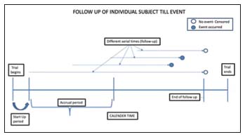
3. Serial Time [Figure 1]: “The duration of the event of interest is called the serial time”

4. Censoring: “it indicates that, time for which a particular patient survives, cannot be measured accurately.” It occurs if:

   1. Something negative happens, i.e., lost to follow-up, drop out, or if the data which is required are unavailable

   2. Something positive happens, i.e., the study ends before the patient has had the predefined event.

5. Interval: “serial time duration of known survival is terminated by predefined event of interest is known as “interval” in K-M analysis.” Only event occurrences define known survival time intervals

6. Survival curve: “defined as the graph of survival S(t) against time t”

7. Time to progression: “time from randomization to disease progression” (death is censored at the time of death or at an earlier visit)

8. Progression free survival: It is defined as the time from randomization to disease progression or death”

9. Time to treatment failure: “A composite end point measuring time from randomization to discontinuation of the treatment for any reason, including disease progression, treatment toxicity, or death”

10. Overall survival (OS): “Defined as time from randomization to death.”

| Figure 1:Illustrates subjects entering a trial and ending at different times. The solid circle represents an event occurrence and the open circles represent censoring

Q4. How Is Kaplan–meier Survival Analysis Plot Prepared?

While preparing for the K-M survival analysis, each patient requires three variables:

1. their serial time [Figure 1]

2. their status (with respect to the event of interest, whether occurred or censored) at the end of their serial time

3. If the study has more than one group, the study group to which they belong. These components may be displayed in [Table 1].

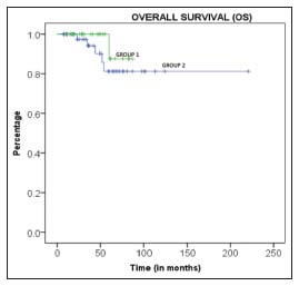
| Figure.2:The survival curve for two groups of patients

Q6. How Are Different Study Groups Compared in Kaplan–meier Survival Analysis?

Log-rank test[3]

• Is the one of the most commonly used tests for comparison of two groups in the survival analysis

• It compares two survival curves using a test with statistical hypothesis

• It uses the null hypothesis indicating that there is no difference between the two population survival curves

• It calculates the Chi-square test at each event time, for each group and then sums up the results

• The summed-up results of each group are added to derive the ultimate Chi-square to compare full curves of each group.

Hazard ratio

• It is similar to the log rank test described above

• However, it has the ratio of hazard rates

• It quantifies the likelihood that a patient will have a hazardous event (negative event) or a hazard during a predefined interval of observation

• Expressed as rate or percentage.

Q7. What Are Different Kaplan–meier Curves Used in Oncology? [4]

1. Overall survival curves

2. Disease-free survival curves

3. Progression-free survival curves.

Q8. What Are Pitfalls of Kaplan–meier Survival Analysis?

1. Must identify the event of interest and units of the measurement along the axes.

2. Shape of the curve:

   1. If too many small steps → a greater number of patients participating

   2. If too large steps → less patients participating.

3. Amount and distribution of censored subject implication

   1. If no censoring: interpret data with caution

   2. If large number of censoring.

      • To question as to why the study was carried out

      • If the treatment was ineffective.

4. The log rank test assumes that the hazard ratio is constant over time.

Conflict of Interest

There are no conflicts of interest.

References

1. Kaplan EL, Meier P. Nonparametric estimation from incomplete observations. Journal of the American Statistical Association 1958; 53: 457-81
2. Rich JT, Neely JG, Paniello RC, Voelker CC, Nussenbaum B, Wang EW. A practical guide to understanding Kaplan-Meier curves. Otolaryngol Head Neck Surg 2010; 143: 331-6
3. Bewick V, Cheek L, Ball J. Statistics review 12: Survival analysis. Crit Care 2004; 8: 389-94
4. Bates S, Fojo T. Assessment of Clinical Response in Cancer DeVita, Hellman, and Rosenberg's Cancer Principles Practice of Oncology. 11th ed. Philadelphia: Wolters Kluwer; 2019

Address for correspondence

Publication History

Received: 31 January 2020

Accepted: 04 June 2020

Article published online:
17 May 2021

© 2020. Indian Society of Medical and Paediatric Oncology. This is an open access article published by Thieme under the terms of the Creative Commons Attribution-NonDerivative-NonCommercial-License, permitting copying and reproduction so long as the original work is given appropriate credit. Contents may not be used for commercial purposes, or adapted, remixed, transformed or built upon. (https://creativecommons.org/licenses/by-nc-nd/4.0/.)

Thieme Medical and Scientific Publishers Pvt. Ltd.
A-12, 2nd Floor, Sector 2, Noida-201301 UP, India

| Figure 1:Illustrates subjects entering a trial and ending at different times. The solid circle represents an event occurrence and the open circles represent censoring

| Figure.2:The survival curve for two groups of patients

References

1. Kaplan EL, Meier P. Nonparametric estimation from incomplete observations. Journal of the American Statistical Association 1958; 53: 457-81
2. Rich JT, Neely JG, Paniello RC, Voelker CC, Nussenbaum B, Wang EW. A practical guide to understanding Kaplan-Meier curves. Otolaryngol Head Neck Surg 2010; 143: 331-6
3. Bewick V, Cheek L, Ball J. Statistics review 12: Survival analysis. Crit Care 2004; 8: 389-94
4. Bates S, Fojo T. Assessment of Clinical Response in Cancer DeVita, Hellman, and Rosenberg's Cancer Principles Practice of Oncology. 11th ed. Philadelphia: Wolters Kluwer; 2019